Extracting Data from Charts and Graphs: The OCR Challenge Solution

Introduction
In today's data-driven world, extracting insights from complex data is essential. Graphs help represent this data, but analyzing them can be challenging, especially for non-experts. The OCR Challenge aimed to develop machine learning solutions for extracting data from graph images and PDFs, making graph analysis more accessible and efficient.
In this blog post, we will cover various data extraction methods, including machine learning models, contour detection, and rule-based methods. We will explore the use of machine learning for extracting data from graph images, examine the role of contour detection and rule-based techniques in data extraction, provide a step-by-step guide to our winning solution, and showcase the effectiveness of our solution with various graph examples.
Join us as we delve into the OCR Challenge and the transformative potential of these data extraction solutions.
Approach
Several different approaches can be used for graph data extraction from images, each with its own advantages and drawbacks. Some common approaches include using machine learning models, contour detection and rule-based methods.
Machine learning models, such as LayoutLMv2, can effectively classify text in graph images and provide insights into the data. However, these models require pre-training and fine-tuning, and may not be effective for all types of graphs.
now, let us see the pros and cons of machine learning models in our use case
pros
Improved accuracy: By automating the process of classifying text in graph images, the LayoutLMv2 model can help to improve the accuracy of the analysis compared to manual classification methods.
Time-saving: The model can analyze graph images faster than humans, reducing the time required for data analysis.
Scalability: The model can be easily scaled to analyze large datasets, making it ideal for applications that involve processing a large volume of graphical data.
Consistency: The model can provide consistent results across multiple images and datasets, eliminating the potential for human error and bias.
cons
Fine-tuning required: Fine-tuning the model on specific datasets may require additional resources and time.
Limitations of the model: The LayoutLMv2 model may not be effective for all types of graph images or data visualizations, and may require additional customization for certain applications.
Interpretability: Machine learning models like the LayoutLMv2 model can be difficult to interpret and explain, making it challenging to understand how the model arrived at its classifications.
Contour detection and Rule-based methods can be a simpler approach that involves detecting the bars or data points in the graph using contour detection, and then Rule-based methods involve defining rules to extract data from the graph image based on its layout and structure. This approach can be effective for specific types of graphs but may require manual customization for each graph type.
Now, let us see the pros and cons of this method
pros
No pre-training required: Unlike machine learning-based methods, contour detection, and basic mathematics does not require pre-training the model on large datasets, which can be time-consuming and computationally intensive.
Relatively simple: The method involves simple calculations that can be easily implemented, making it accessible to a wide range of users and applications.
Works for simple graphs: This method can be effective for simple graphs with clear and distinct bars and labels.
cons
Limited applicability: This method may not work effectively for more complex graphs with overlapping bars or multiple datasets.
Susceptible to errors: The accuracy of the method can be affected by errors in contour detection or OCR, which can result in the misclassification of text labels.
Lack of flexibility: The method may not be easily adaptable to different types of graphs or applications, as it relies on specific calculations and assumptions about the layout of the graph.
Now, we will discuss both of these methods in detail one by one.
Machine learning model
LayoutLMv2 is a powerful machine learning model developed by Microsoft that is specifically designed to analyze document layouts. This model uses a combination of computer vision techniques and natural language processing (NLP) to understand the structure and content of documents, allowing it to identify key elements such as titles, captions, tables, and graphs.
LayoutLMv2 can be used to finetune a machine learning model to classify the text in a graph image into categories such as title, x-axis, y-axis, and legends. The first step in using LayoutLMv2 for graph analysis is to collect a large dataset of graph images and their associated labels. The labels should include information about the location and content of each element in the graph, such as the title, x-axis label, y-axis label, and legend.
This dataset can be created manually by labeling each graph image. the model can then be fine-tuned using the created dataset of labeled graphs, allowing it to adapt to our use cases. (you can see the sample of the dataset I created here : ShubhamMehla3/graph-ocr/dataset.zip)
Let's take a look at the code for fine-tuning our machine-learning model. The following code is just a sample (you can find the actual working code on my GitHub, https://github.com/ShubhamMehla3/graph-ocr/blob/main/run_seq_labeling.py ).
from layoutlm import LayoutlmConfig, LayoutlmForTokenClassification
from transformers import BertTokenizer,AdamW
from torch.utils.data import DataLoader, RandomSampler
import torch
from tqdm import tqdm, trange

MODEL_CLASSES = { "layoutlm": (LayoutlmConfig, LayoutlmForTokenClassification, BertTokenizer), }

def train( train_dataset, model, tokenizer, labels, pad_token_label_id):

    """ Train the model """
    if torch.cuda.is_available():
        device = torch.device("cuda")
        print("GPU is available")
    else:
        device = torch.device("cpu")
        print("GPU is not available, using CPU instead")

    train_sampler = RandomSampler(train_dataset)
    train_dataloader = DataLoader(train_dataset, sampler=train_sampler,                batch_size=args.train_batch_size, collate_fn=None )
    no_decay = ["bias", "LayerNorm.weight"]
    optimizer = AdamW( lr=learning_rate, eps=adam_epsilon)
    model = torch.nn.Module(model, find_unused_parameters=True)

    global_step, tr_loss = 0, 0.0
    model.zero_grad()
    train_iterator = trange(num_train_epochs, desc="Epoch")
    for in trainiterator:
        epoch_iterator = tqdm(train_dataloader, desc="Iteration")
        for step, batch in enumerate(epoch_iterator):
            model.train()
            inputs = {"input_ids": batch[0].to(device), "attention_mask": batch[1].to(device),     "labels": batch[3].to(device)}
            inputs["bbox"] = batch[4].to(device)
            inputs["token_type_ids"] = batch[2].to(device)

    outputs = model(**inputs)
    loss = outputs[0]
    loss.backward()
    tr_loss += loss.item()

    optimizer.step()
    # scheduler.step() # Update learning rate schedule
    model.zero_grad()
    global_step += 1

    return global_step, tr_loss / global_step
The train() function takes as input the train_dataset, model, tokenizer, labels, and pad_token_label_id.The function first checks if a GPU is available and sets the device accordingly. It then creates a RandomSampler for the training dataset and a DataLoader using the RandomSampler, with a batch size of train_batch_size. The function then initializes an AdamW optimizer with a learning rate of learning_rate and an epsilon value of adam_epsilon. The model is then called with the input tensors, and the output loss is computed and backpropagated through the model. The training loop continues for num_train_epochs epochs, with a progress bar for each epoch and iteration. At the end of each epoch, global_step and tr_loss variables are updated. The function returns the final global_step and the average training loss per step.
from layoutlm import FunsdDataset, LayoutlmConfig, LayoutlmForTokenClassification
from transformers import BertTokenizer
import torch

MODEL_CLASSES = { "layoutlm": (LayoutlmConfig, LayoutlmForTokenClassification, BertTokenizer), }


def main():

    if torch.cuda.is_available():
        device = torch.device("cuda")
        print("GPU is available")
    else:
        device = torch.device("cpu")
        print("GPU is not available, using CPU instead")

    labels = get_labels(labels) # in our case labels will be x-axis,y-axis,title
    num_labels = len(labels) # Use cross entropy ignore index as padding label id so that only real     label ids contribute to the loss later
    pad_token_label_id = CrossEntropyLoss().ignore_index

    config = config_class.from_pretrained( "layoutlm-base-uncased/", num_labels=num_labels,force_download = True, ignore_mismatched_sizes=True, cache_dir= cache_dir_path else None)

    tokenizer = tokenizer_class.from_pretrained( "microsoft/layoutlm-base-uncased",do_lower_case=True, force_download = True, ignore_mismatched_sizes=True, cache_dir= cache_dir_path else None)

    model = model_class.from_pretrained( "layoutlm-base-uncased/", config=config)

    model.to(args.device)

    train_dataset = FunsdDataset( args, tokenizer, labels, pad_token_label_id, mode="train" )

    global_step, tr_loss = train( args, train_dataset, model, tokenizer, labels, pad_token_label_id )

    tokenizer = tokenizer_class.from_pretrained( "microsoft/layoutlm-base-uncased",force_download = True, do_lower_case=args.do_lower_case, ignore_mismatched_sizes = True)

    model = model_class.from_pretrained(args.output_dir)
    model.to(args.device)
    result, predictions = evaluate( args, model, tokenizer, labels, pad_token_label_id, mode="test" )

    return result,predictions
The main() function reads the dataset then finetune our layoutlmv2 model on the dataset we created along with calculating the loss on training and the test data.
Flow of the main() function goes like : it then calls the get_labels() function to get the list of labels for the token classification task. The number of labels is computed and the padding label id is set to the CrossEntropyLoss().ignore_index. The function then initializes a LayoutlmConfig with the number of labels and downloads the pre-trained LayoutLM-base-uncased model. A LayoutlmForTokenClassification model is initialized using the downloaded LayoutlmConfig. The train_dataset is created using the FunsdDataset class and the train() function is called to train the model. The function then downloads the pre-trained BertTokenizer and initializes a new LayoutlmForTokenClassification model from the output directory. The evaluate() function is called to evaluate the trained model on the test dataset, and the function returns the evaluation result and predictions.
In conclusion, LayoutLMv2 is a powerful machine-learning model that can be used to finetune a model for classifying text in graph images. This method can provide valuable insights into the structure and content of graphs, making it easier to analyze and understand complex data. As the amount of data available continues to grow, LayoutLMv2 will become an increasingly important tool for businesses and organizations looking to gain insights from their data.
Contour detection and Rule-based methods
In addition to using LayoutLMv2, another method for analyzing graphs is to use contour detection and basic mathematics to classify the text extracted from the image. This method is particularly useful for analyzing bar charts, where the bars themselves are the primary means of conveying information.
The first step in this method is to use computer vision techniques to detect the bars in the graph image. This can be done using contour detection, which identifies the outlines of objects in an image. Once the bars have been detected, the height and position of each bar can be extracted using basic mathematics.
Once the heights and positions of the bars have been extracted, the next step is to identify the labels for the x-axis and y-axis. This can be done using NLP techniques to analyze the text in the graph image. The labels for the x-axis and y-axis can then be mapped to the corresponding bars using the positions of the bars and the position of the labels.
You can find the working for this from this colab notebook : https://github.com/ShubhamMehla3/graph-ocr/blob/main/inference.ipynb
To test this code you can also download the horizontal bar graph image from here :
https://github.com/ShubhamMehla3/graph-ocr/tree/main/images
Code Walkthrough
Using contour detection to detect all the bars present in the graph image. To enhance the effectiveness of the contour detection algorithm for detecting all the bars present in the graph image, several filters can be applied. These filters can help to improve the accuracy and quality of the contour detection results. Examples of filters that can be utilized include Gaussian smoothing, thresholding, and edge detection. Gaussian smoothing can help to reduce noise and unwanted details in the image, while thresholding can help to segment the image into distinct regions based on pixel intensity. Edge detection, on the other hand, can help to identify the boundaries of the bars and other features present in the image. By employing such filters, the contour detection algorithm can be made more robust and accurate in detecting all the bars present in the graph image.
def calc_contours(image_path):
  img = cv2.imread(image_path)

  # Apply bilateral filter
  img_bilateral = cv2.bilateralFilter(img, 9, 75, 75)

  # Convert the image to grayscale
  gray = cv2.cvtColor(img, cv2.COLOR_BGR2GRAY)

  # Apply thresholding to remove text and noise
  _, thresh = cv2.threshold(gray, 150, 255, cv2.THRESH_BINARY)

  # Apply ROI masking to exclude non-graph regions
  mask = np.zeros_like(thresh)
  mask[50:400, 100:700] = 255
  masked_thresh = cv2.bitwise_and(thresh, mask)

  # Apply edge detection using the Canny algorithm
  edges = cv2.Canny(gray, 100, 200)

  # Apply horizontal line detection using HoughLinesP
  lines = cv2.HoughLinesP(edges, 1, np.pi/180, 100, minLineLength=250, maxLineGap=15)
  horizontal_lines = []
  for line in lines:
      x1, y1, x2, y2 = line[0]
      if abs(y1 - y2) < 5: # Check if the line is horizontal
          horizontal_lines.append(line)

  # Draw the detected lines on the image
  for line in horizontal_lines:
      x1, y1, x2, y2 = line[0]
      # cv2.line(img, (x1, y1), (x2, y2), (255, 255, 255), 2)

  # Find contours in the image
  contours, hierarchy = cv2.findContours(edges, cv2.RETR_TREE, cv2.CHAIN_APPROX_SIMPLE)

  # Filter out unwanted contours based on contour area and aspect ratio
  bars = []
  for cnt in contours:
      area = cv2.contourArea(cnt)
      x, y, w, h = cv2.boundingRect(cnt)
      aspect_ratio = float(w) / h
      if area > 7 and aspect_ratio > 5 and aspect_ratio < 50000:
          bars.append(cnt)

  ###### 2 consecutive element from the bars represent single contour only
  ###### and we will consider only one of them, so we will filter out odd index elemnts from the "bars"

  def filter_bars(bars):
    lst = []
    for i in range(len(bars)):
      if(i%2==1):
        lst.append(bars[i])
    return lst

  bars = filter_bars(bars)

  # Draw the remaining contours on the image
  cv2.drawContours(img, bars, -1, (255, 255, 0), 2)

  # Show the image
  cv2_imshow(img)
  return bars
I am utilizing the output of LayoutLMv2 (without any fine-tuning), a pre-trained language and layout model, to obtain the coordinates of all the extracted text. This approach has yielded superior results compared to using Pytesseract without any fine-tuning.
def loadFromLayoutlmv2():
  feature_extractor = LayoutLMv2FeatureExtractor.from_pretrained("microsoft/layoutlmv2-base-uncased")# apply_ocr is set to True by default
  tokenizer = LayoutLMv2TokenizerFast.from_pretrained("microsoft/layoutlmv2-base-uncased")
  model = LayoutLMv2ForTokenClassification.from_pretrained("nielsr/layoutlmv2-finetuned-funsd")
  return feature_extractor,tokenizer,model

def labelForBoxes():
  dataset = load_dataset("nielsr/funsd", split="test")
  # define id2label, label2color
  labels = dataset.features['ner_tags'].feature.names
  id2label = {v: k for v, k in enumerate(labels)}
  label2color = {'question':'blue', 'answer':'green', 'header':'orange', 'other':'violet'}
  return id2label, label2color

def unnormalize_box(bbox, width, height):
     return [
         width * (bbox[0] / 1000),
         height * (bbox[1] / 1000),
         width * (bbox[2] / 1000),
         height * (bbox[3] / 1000),
     ]

def iob_to_label(label):
    label = label[2:]
    if not label:
      return 'other'
    return label

def process_image(image,id2label,label2color,feature_extractor,tokenizer,model):

    # Convert the image to RGB format
    image = image.convert('RGB')
    width, height = image.size

    # get words, boxes
    encoding_feature_extractor = feature_extractor(image, return_tensors= "pt")
    words, boxes = encoding_feature_extractor.words, encoding_feature_extractor.boxes
    # encode
    encoding = tokenizer(words, boxes=boxes, truncation=True, return_offsets_mapping=True, return_tensors="pt")
    offset_mapping = encoding.pop('offset_mapping')
    encoding["image"] = encoding_feature_extractor.pixel_values
    # forward pass
    outputs = model(**encoding)
    # get predictions
    predictions = outputs.logits.argmax(-1).squeeze().tolist()
    token_boxes = encoding.bbox.squeeze().tolist()
    # only keep non-subword predictions
    is_subword = np.array(offset_mapping.squeeze().tolist())[:,0] != 0
    true_predictions = [id2label[pred] for idx, pred in enumerate(predictions) if not is_subword[idx]]
    true_boxes = [unnormalize_box(box, width, height) for idx, box in enumerate(token_boxes) if not is_subword[idx]]
    # draw predictions over the image
    draw = ImageDraw.Draw(image)
    font = ImageFont.load_default()
    for prediction, box in zip(true_predictions, true_boxes):
        predicted_label = iob_to_label(prediction).lower()
        draw.rectangle(box, outline=label2color[predicted_label])
        draw.text((box[0]+10, box[1]-10), text=predicted_label, fill=label2color[predicted_label], font=font)
    return image,true_boxes,words,true_predictions,true_boxes,is_subword
After , this I performed the rule-based method to get the results. Basically, i just write a couple of mathematical operations.
First of all the, all the coordinates of the text is normalized because We want to write the generalize code .
######## scaled data #############


def normalize_bbox(bboxes,img):
  # removing the fist and last coordinates
  bboxes= bboxes[1:-1]

  # Define the new image size
  new_width = 100
  new_height = 100

  original_width,original_height = img.size
  # Calculate the scaling factors
  x_scale = new_width / original_width
  y_scale = new_height / original_height

  #parsing the bboxes
  new_bboxes = []
  for bbox in bboxes:
    x1,y1,x2,y2 = bbox
    # Normalize the bounding box coordinates
    new_x1 = int(x1 * x_scale)
    new_y1 = int(y1 * y_scale)
    new_x2 = int(x2 * x_scale)
    new_y2 = int(y2 * y_scale)

    new_bbox = new_x1,new_y1,new_x2,new_y2
    new_bboxes.append(new_bbox)
  return new_bboxes
The extracted text is segregated into three categories based on their coordinates, namely, heading, keys (y-axis), and values (representing the bars in the bar graph). To standardize the bounding box, a normalization process is carried out. The categorization is carried out using a certain concept: for y-axis text, the y-coordinate of their bounding box does not vary much (a basic mathematical principle).
The text in the values category is assigned to the nearest bar, while the text in the keys category is also assigned to the nearest bar. Based on the outcomes of the preceding two points, the keys (y-axis) text is matched with the corresponding values (bars in the graph).
######### categorize the words into "keys, values, headers"

def graph_categorizer(words,bboxes,img):

  output_dict = {"headers":[],"keys":[],"values":[]}

  bboxes = normalize_bbox(bboxes,img)

  for idx in range(len(words[0])):
    x1,y1,x2,y2 = bboxes[idx]
    ###### header
    if(y2<=13):
      output_dict['headers'].append(words[0][idx])
    ###### keys
    elif(x2<43):
      output_dict['keys'].append(words[0][idx])
    ###### values
    elif(x2>=43):
      output_dict['values'].append(words[0][idx])

  return output_dict

####### assign values to their respective keys with the help contours


def nearest_assignment(updated_categorized_data,updated_words_to_bboxes,contours_right_coords):
  #### values to contour relation
  contour_to_values = {}
  for idx in range(len(contours_right_coords)):
    contours = contours_right_coords[idx]
    cont_x,_ = contours
    min_dist = float('inf')
    min_value = None
    for value in updated_categorized_data['values']:
      _,_,value_x,_ = updated_words_to_bboxes[value]
      curr_dist = abs(value_x-cont_x)
      # print(value,curr_dist,value_x,cont_x)
      if(min_dist>curr_dist):
        min_dist = curr_dist
        min_value = value
    contour_to_values[contours[1]] = min_value


  ######## 2nd method
  if(len(updated_categorized_data['values'])==len(contours_right_coords)):
    contour_to_values = {}
    for idx in range(len(contours_right_coords)):
      contours = contours_right_coords[idx]
      contour_to_values[contours[1]] = updated_categorized_data['values'][idx]
  return contour_to_values

#### assign values to their respective keys

def assign_value_to_keys(updated_categorized_data,updated_words_to_bboxes,contours_right_coords,contour_to_values):

  # fist assign the keys to the bars
  bars_to_keys = {}

  ## parsing the updated_categorized_data
  for cnt in contours_right_coords:
    _,cond_y = cnt
    min_diff = float('inf')
    right_key = None
    for key in updated_categorized_data['keys']:
      _,_,_,y = updated_words_to_bboxes[key]
      diff = float(abs(cond_y - y))
      if(min_diff > diff):
        min_diff = diff
        right_key = key
    bars_to_keys[cond_y] = right_key


  ###### simple solution for bars to keys
  if(len(contours_right_coords)==len(updated_categorized_data['keys'])):
    bars_to_keys = {}
    for idx in range(len(contours_right_coords)):
      contours = contours_right_coords[idx]
      bars_to_keys[contours[1]] = updated_categorized_data['keys'][idx]


  # now assigning the keys to the values
  keys_to_values = {}
  for k,v in bars_to_keys.items():
    keys_to_values[v] = contour_to_values[k]

  return keys_to_values
Sample Outputs
output 1
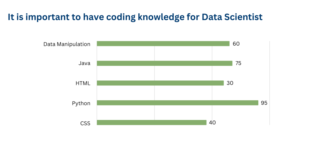
input image :
output :
{'header': ['It is important to have coding knowledge for Data Scientist'],
'Mapping': {'Data Manipulation': '60',
'Java': '75',
'HTML': '30',
'Python': '95'}}
observation :
our model was not able to detect the last horizontal bar (CSS). For the rest, it was working fine.
output 2
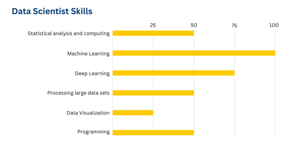
One issue with the OCR I am using is that sometimes it is not able to detect the numerical values. Same Happened with this graph.
ouput :
{'header': ['Data Scientist Skills'],
'Mapping': {'Statistical analysis and computing': '100',
'Machine Learning': '100',
'Processing large data sets': '100',
'Data Visualization': '100',
'Programming' : '100'
}}
observation :
OCR only extracted one numerical value from the image i.e. 100 and hence all the values from the y-axis got mapped to 100.
output 3
input image :

output :
{'Skills Of Coding For Begineer' : 'JavaScript' }
output 4
input image :

output :
{'skills Of Coding For Intermediate' : 'PHP' }
Conclusion
In conclusion, contour detection and basic mathematics can be useful approaches for classifying text in graph images, especially for simple graphs with clear and distinct bars and labels. However, the method has limitations regarding its applicability to more complex graphs, susceptibility to errors, and lack of flexibility for different types of graphs and applications.
Further Reading
If you enjoyed this blog post on the OCR Challenge and its innovative solutions, we invite you to read more about the applications of OCR technology combined with GPT-4 in our other blog posts, where we cover OCR for images, PDFs, table extraction, and entity recognition:
OCR using Amazon Textract and GPT-4: Dive into the integration of Amazon Textract and GPT-4 for OCR applications, exploring how these technologies can be combined to enhance data extraction and text analysis for images, PDFs, tables, and entities.
OCR using Google Vision API and GPT-4: Learn how the powerful combination of Google Vision API and GPT-4 can transform OCR capabilities, providing accurate and efficient data extraction from images, documents, tables, and entities.
OCR using Azure API and GPT-4: Discover the potential of leveraging Azure API and GPT-4 for OCR tasks, improving the analysis of text and data from various sources, including images, PDFs, tables, and entity recognition.
By exploring these additional blog posts, you will gain a deeper understanding of the different OCR technologies and their potential when combined with GPT-4, further expanding your knowledge of data extraction from charts, graphs, and other sources.
To learn about more interesting and cool NLP and LLM Applications, look into our other Blogs and YouTube channel.
Also, want to learn about the state-of-the-art stuff in AI? Don't forget to subscribe to AI Demos. A place to learn about the latest and cutting-edge tools in AI!
